
Isochrones in Stockholm
15 Jan 2021
Suppose that you are about to relocate. An important factor in deciding where to is the time it takes to travel to work (well, at least in non-pandemic times). One proxy for this is of course distance – move to a place that is close to your workplace. However, it is clearly not a perfect one: the time to travel from one location to another depends heavily on the available means of transport, the location of roads and public transport, etc.
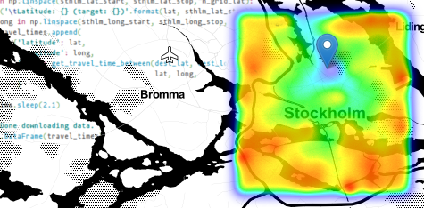
One way to illustrate this is by drawing isochrones on a map:
An isochrone (iso = equal, chrone = time) is defined as “a line drawn on a map connecting points at which something occurs or arrives at the same time”.
However, since Stockholm is far from a flat field – it is situated on 14 islands – the determination of isochrones (and, in turn, the relocation problem) is somewhat non-trivial.
A quick Google search shows that there are several services available that can plot isochrones, but, as far as I can tell, most of these are based on transportation by bicycle or car (e.g., RouteWare and Iso4App). The ones that include travel by train or public transport are either specific to larger cities in Europe (e.g., Tom Carden and Mapumental for London, TravelTime, Mapnificent and Targomo) or operate on a much coarser scale than the inner city of Stockholm (e.g., Empty Pipes and CityMonitor.ai) .
As a fun weekend project, let us see if we can put together our own solution that allows us to plot a travel-time map (isochrones) of Stockholm.
Time to travel from A to B
Public transport (metro, buses, trams) in the inner city of Stockholm is handled by SL. On their website, you can get the best route (along with an estimate of the travel time) between any two locations in Stockholm. Thanks to the people at Trafiklab, it is possible to access this programmatically through an API.
As a first step, we register at Trafiklab and request an API-key to the SL
Reseplanerare 3.1 API. I have
saved the key in a text-file called sl_api_key.txt:
with open('sl_api_key.txt') as f:
    api_key = f.read()
The API is documented here. Our first goal will be to write a function that returns the travel time between any two coordinates in Stockholm (once we have this, we can query this function over a grid).
Querying the API
A query to the
Trip-API
requires us to specify the API-key, an origin and a destination (either as
a station name, or with latitude and longitude coordinates). We can optionally
specify a date and time for the trip (since we are optimizing travel times to
and from work, we probably want to specify a weekday around rush hour) and if we
want to leave or arrive by that time (searchForArrival). We can also specify
how many trip suggestions that we want with numF and numB – for us, just
one is sufficient. The query returns JSON
data with each trip suggestion, and the details on each “segment” (Leg) of the
trip.
The first segment is usually a walk to the nearest station, the intermediate segments different modes of transportation (metro, bus, etc.), and the last segment a walk from a final stop to the destination’s coordinates.
For some reason, the duration-field of some segments is sometimes not included
in the returned data, which causes an incorrect estimate of the total duration
of the trip. As a workaround for this, we can manually compute the travel time
by subtracting the departure time from the arrival time. The departure time is
specified in the Date and Time fields of the first segment of the trip, and
the arrival time in the Date and Time fields of the last segment. These are
given as strings, so let us first make a helper function to convert these
strings to a datetime object – this will make it easier to compute the
time-difference (i.e., travel time).
from datetime import datetime

def strs_to_datetime(date_str, time_str):
    return datetime.strptime(date_str + ' ' + time_str, '%Y-%m-%d %H:%M:%S')

strs_to_datetime('2021-01-15', '13:30:00')
datetime.datetime(2021, 1, 15, 13, 30)
In the function below, we construct a query for the API, parse the returned data (compute the travel time manually) and return the travel time (in minutes) between two coordinates. We use Monday 18 January 2021 at 08:00 as our arrival time and we only ask for one trip suggestion.
import requests

def get_travel_time_between(origin_lat, origin_long, dest_lat, dest_long,
                            verbose = False):

    params = {
        'key': api_key,
        'originCoordLat': origin_lat,
        'originCoordLong': origin_long,
        'destCoordLat': dest_lat,
        'destCoordLong': dest_long,
        'date': '2021-01-18',
        'time': '08:00',
        'searchForArrival': 1, # arrive(1)/depart(0) by specified date and time
        'numF': 0,             # trip suggestions after specified date and time
        'numB': 0              # trip suggestions before specified  -- "" --
    }

    response = requests.get('http://api.sl.se/api2/TravelplannerV3_1/trip.json',
                            params=params)

    # make sure data was retreived successfully
    if not response.status_code == 200:
        if verbose:
            print('ERROR ({}) in retrieving time between ({}, {}) and ({}, '
                  '{})!'.format(response.status_code,
                                origin_lat,
                                origin_long,
                                dest_lat,
                                dest_long)
                  )
        return -1

    json_data = response.json()

    if not 'Trip' in json_data:
        if verbose:
            print('\t\tERROR: \'Trip\' not in returned json-data!')
        return -1

    if len(json_data['Trip']) > 1:
        if verbose:
            print('\t\tWARNING: Received more than 1 trip suggestion!')

    # the returned trip-duration is sometimes incorrectly computed by
    # the API, so let's compute it manually as the time-delta between
    # the first and the last segment of the trip
    first_segment = json_data['Trip'][0]['LegList']['Leg'][0]
    last_segment  = json_data['Trip'][0]['LegList']['Leg'][-1]

    start_time = strs_to_datetime(first_segment['Origin']['date'],
                                  first_segment['Origin']['time'])

    end_time = strs_to_datetime(last_segment['Destination']['date'],
                                last_segment['Destination']['time'])

    return (end_time - start_time).total_seconds() / 60
Let us see if it works. Consider, for example, the travel time between KTH and Liljeholmen (which, I know should be roughly half an hour). The coordinates can be obtained using Google Maps.
kth_lat  = 59.3486016
kth_long = 18.0690764

liljeholmen_lat  = 59.3113696
liljeholmen_long = 18.0236446

get_travel_time_between(kth_lat, kth_long, liljeholmen_lat, liljeholmen_long)
31.0
So, 31 minutes – that sounds about right!
Travel times within Stockholm
Now that we can compute the travel time between any two coordinates, let us do it over a grid ontop of Stockholm. This will then allow us to estimate isochrones (as the level sets of the data).
With the free API, we are
allowed to do 10,000 queries
per month, and a maximum of 30 per minute. This translates to one query every
other second – in the code below, we sleep a bit longer (2.1 seconds) for
some extra margin (28 queries per minute). We let the grid span over a rectangle
from
Barkaby
in the north-west, down to
Älta
in the south-east. This, roughly, covers central Stockholm.
import pandas as pd
import numpy as np
import time

# Barkaby
sthlm_lat_start  = 59.4085823
sthlm_long_start = 17.8542054

# Älta
sthlm_lat_stop  = 59.2563638
sthlm_long_stop = 18.1744499

def get_travel_times_to(dest_lat, dest_long):

    # number of gridpoints
    n_grid_lat  = 40
    n_grid_long = 40

    print('Will do {} API queries...'.format(n_grid_lat * n_grid_long))
    print('Expected time to finish: {:.1f} m\n'.format(n_grid_lat *
                                                       n_grid_long * 2.1 / 60))
    travel_times = []
    for lat in np.linspace(sthlm_lat_start, sthlm_lat_stop, n_grid_lat):
        print('\tLatitude: {}'.format(lat))
        for long in np.linspace(sthlm_long_start, sthlm_long_stop, n_grid_long):
            travel_times.append(
                {'latitude': lat,
                 'longitude': long,
                 'time': get_travel_time_between(lat, long,
                                                 dest_lat, dest_long)
                 }
            )
            # rate-limit is 30 queries / minute --> 1 query / 2 seconds
            time.sleep(2.1)

    print('\nDone downloading data.')
    return pd.DataFrame(travel_times)
Suppose we work at KTH (at the Division of Decision and
Control Systems :) with lat = 59.349725, long
= 18.0660567. Then we can download all travel times from points on the grid by
calling the function we defined above:
work_lat  = 59.349725
work_long = 18.0660567

travel_df = get_travel_times_to(work_lat, work_long)
Will do 1600 API queries...
Expected time to finish: 56.0 m

	Latitude: 59.4085823
	Latitude: 59.40467926153846
	Latitude: 59.400776223076925
	Latitude: 59.39687318461539
	Latitude: 59.39297014615384
	Latitude: 59.389067107692306
	Latitude: 59.38516406923077
	Latitude: 59.38126103076923
	Latitude: 59.377357992307694
	Latitude: 59.37345495384616
	Latitude: 59.36955191538461
	Latitude: 59.365648876923075
	Latitude: 59.36174583846154
	Latitude: 59.3578428
	Latitude: 59.35393976153846
	Latitude: 59.350036723076926
	Latitude: 59.34613368461539
	Latitude: 59.342230646153844
	Latitude: 59.33832760769231
	Latitude: 59.33442456923077
	Latitude: 59.33052153076923
	Latitude: 59.326618492307695
	Latitude: 59.32271545384616
	Latitude: 59.31881241538461
	Latitude: 59.314909376923076
	Latitude: 59.31100633846154
	Latitude: 59.3071033
	Latitude: 59.303200261538464
	Latitude: 59.29929722307693
	Latitude: 59.29539418461539
	Latitude: 59.291491146153845
	Latitude: 59.28758810769231
	Latitude: 59.28368506923077
	Latitude: 59.27978203076923
	Latitude: 59.275878992307696
	Latitude: 59.27197595384616
	Latitude: 59.268072915384614
	Latitude: 59.26416987692308
	Latitude: 59.26026683846154
	Latitude: 59.2563638

Done downloading data.
So what did we just download?
travel_df.describe()
| latitude | longitude | time | |
|---|---|---|---|
| count | 1600.000000 | 1600.000000 | 1600.000000 |
| mean | 59.332473 | 18.014328 | 52.476250 |
| std | 0.045068 | 0.094817 | 16.056636 |
| min | 59.256364 | 17.854205 | -1.000000 |
| 25% | 59.294418 | 17.934267 | 43.000000 |
| 50% | 59.332473 | 18.014328 | 52.000000 |
| 75% | 59.370528 | 18.094389 | 60.000000 |
| max | 59.408582 | 18.174450 | 123.000000 |
Or, if we visualize the last column (the travel times from different locations in Stockholm to our workplace):
import matplotlib
travel_df['time'].plot.hist(bins=45)
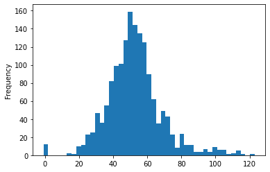
As can be seen from the table and the graph above, there were a few queries for which the
API returned an error (and, hence, time = -1). For now, let us just drop these and leave
it to future work to investigate why.
travel_df = travel_df[travel_df['time'] != -1]
travel_df.shape
(1588, 3)
So (1600 - 1588) = 12 entries were removed – not that many.
Plotting travel times
Now that we have the data (coordinates and the associated travel times to our workplace), let us try to visualize it in some useful way.
We can plot the data directly using, for example, Matplotlib:
import matplotlib.pyplot as plt

fig = plt.figure(figsize = (7,7), dpi = 90)
ax = fig.add_subplot(111, projection = '3d')

ax.scatter(travel_df['latitude'],
           travel_df['longitude'],
           travel_df['time'],
           c = travel_df['time'],
           s = 8)

ax.set_xlabel('latitude')
ax.set_ylabel('longitude')
ax.set_zlabel('travel time [min]')
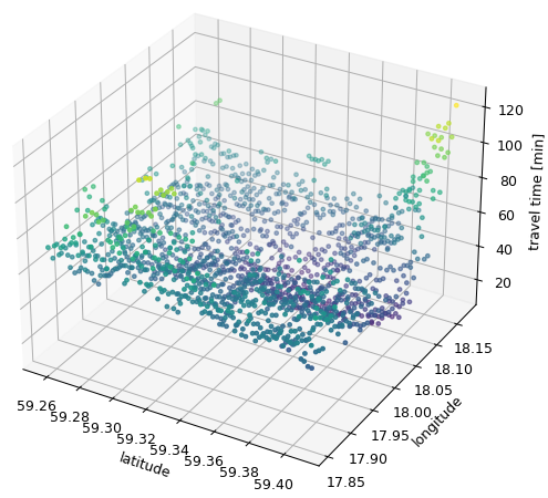
Interesting – but, perhaps it would be easier to interpret if we rotated the viewport to coincide with how a map is normally drawn (north pointing up, east to the right) and changed the colormap?
fig = plt.figure(figsize = (7,7), dpi = 90)
ax = fig.add_subplot(111, projection = '3d')

ax.scatter(travel_df['latitude'],
           travel_df['longitude'],
           travel_df['time'],
           c = travel_df['time'],
           s = 8,
           cmap = matplotlib.cm.jet)

# rotate viewport
ax.view_init(90, 0)
ax.invert_xaxis()

ax.set_zticklabels([])

ax.set_xlabel('latitude')
ax.set_ylabel('longitude')
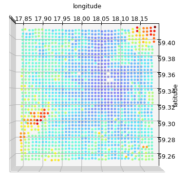
Slightly better. But there is still some crucial information missing for it to be informative – at least I do not have a very good intuition for what latitude and longitude correspond to where in Stockholm.
Plotting on a map
Instead, we would like to use something with specialized map-plotting functionality. A quick Google search yields a number of Python-libraries that provide such functionality: Matplotlib Basemap, Folium, Plotly, etc.
Below, I use Folium since it has easy to use support for drawing nice looking heatmaps (which is essentially what we plotted above when we rotated the viewport).
import folium
from folium.plugins import HeatMap

def plot_time_map(additional_markers = [], data = travel_df):
    map = folium.Map(
        location = [(sthlm_lat_start + sthlm_lat_stop) / 2,
                    (sthlm_long_start + sthlm_long_stop) / 2],
        tiles='Stamen Toner',
        zoom_start=11
    )

    marker_str = 'Work'
    folium.Marker([work_lat, work_long],
                  popup=marker_str,
                  tooltip=marker_str).add_to(map)

    for marker in additional_markers:
        folium.Marker([marker['latitude'],
                       marker['longitude']],
                       popup=marker['string'],
                       icon=folium.Icon(color='red'),
                       tooltip=marker['string']).add_to(map)


    max_time = data['time'].max()

    HeatMap(data.to_numpy(),
            min_opacity=0.1,
            max_val=max_time,
            radius=11,
            blur=11,
            max_zoom=10
            ).add_to(map)

    return map
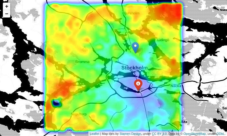
Then we can plot the travel-time data on a map of Stockholm with:
plot_time_map()
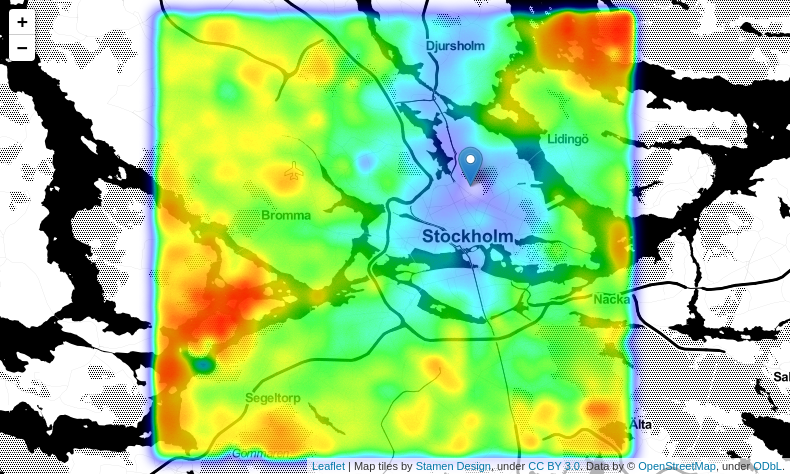
Note that our workplace (i.e., KTH) has been marked with a blue marker.
Cool. So what can we do with this now?
Distance vs travel time
Consider, for example, Ropsten (north-east of KTH) and Liljeholmen (south-west of KTH):
ropsten_lat  = 59.357298
ropsten_long = 18.1000293

plot_time_map([{'latitude': ropsten_lat,
                'longitude': ropsten_long,
                'string': 'Ropsten'},
               {'latitude': liljeholmen_lat,
                'longitude': liljeholmen_long,
                'string': 'Liljeholmen'}])
Even though Liljeholmen is more than twice as far away from KTH as Ropsten is (as measured by the bird path, in meters):
from geopy import distance

print('Distance to')
print('\tRopsten:\t', end='')
print(distance.distance((work_lat, work_long),
                        (ropsten_lat, ropsten_long)))

print('\tLiljeholmen:\t', end='')
print(distance.distance((work_lat, work_long),
                        (liljeholmen_lat, liljeholmen_long)))
Distance to
	Ropsten:	2.1086527827170345 km
	Liljeholmen:	4.907707524415635 km
The travel time (using public transport) is almost the same:
print('Travel time from')
print('\tRopsten: ', end='')
print('\t{:.0f} min'.format(get_travel_time_between(ropsten_lat,
                                                    ropsten_long,
                                                    work_lat,
                                                    work_long)))

print('\tLiljeholmen: ', end='')
print('\t{:.0f} min'.format(get_travel_time_between(liljeholmen_lat,
                                                    liljeholmen_long,
                                                    work_lat,
                                                    work_long)))
Travel time from
	Ropsten: 	28 min
	Liljeholmen: 	33 min
The reason is that to go from Ropsten, one has to first take the metro to Östermalmstorg and there change line, whereas from Liljeholmen it is straight with no changes.
In other words, just because something is closer on the map does not mean it is “closer in time”.
Isochrones
So what about the isochrones? They can be read from the earlier plots. However, we can make them more explicit by plotting only the locations from which our workplace can be reached within a certain number of minutes.
def plot_isochrone(time):
    isochrone = travel_df[travel_df['time'] <= time]

    map = folium.Map(
        location = [(sthlm_lat_start + sthlm_lat_stop) / 2,
                    (sthlm_long_start + sthlm_long_stop) / 2],
        tiles='Stamen Toner',
        zoom_start=11
    )

    marker_str = 'Work'
    folium.Marker([work_lat, work_long],
                  popup=marker_str,
                  tooltip=marker_str).add_to(map)

    HeatMap(isochrone[['latitude', 'longitude']].to_numpy(),
            min_opacity=0.5,
            max_val=time,
            radius=11,
            blur=11,
            max_zoom=10,
            gradient={1.0:'#00AA00', 0.0:'#00FF00'}
            ).add_to(map)

    return map
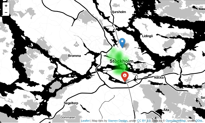
25-minute isochrone
Hence, all the locations from which KTH can be reached within 25 minutes on a Monday morning are:
plot_isochrone(25)
35-minute isochrone
Similarly, all the locations from which it can be reached within 35 minutes are:
plot_isochrone(35)
Depending on our threshold for travel time to work, these plots give us a good indication of areas that would be suitable for relocating to.
More than one point of interest
Suppose now that there is more than one point of interest. You might have some
location-specific hobby which you would also like to minimize travel time to, or your
partner might want to live close to work as well. How can we find the locations from which
both work_lat, work_long and hobby_lat, hobby_long can be reached within some given
time-threshold (that is, what are the locations that should be considered for
relocation)?
We can solve this by intersecting the isochrones for the two destinations. First, let us download travel-time data for the location of the hobby (here, I use Eriksdalsbadet as an example):
hobby_lat  = 59.3048988
hobby_long = 18.0733449

hobby_df = get_travel_times_to(hobby_lat, hobby_long)

hobby_df = hobby_df[hobby_df['time'] != -1]
Will do 1600 API queries...
Expected time to finish: 56.0 m

	Latitude: 59.4085823
	Latitude: 59.40467926153846
	Latitude: 59.400776223076925
	Latitude: 59.39687318461539
	Latitude: 59.39297014615384
	Latitude: 59.389067107692306
	Latitude: 59.38516406923077
	Latitude: 59.38126103076923
	Latitude: 59.377357992307694
	Latitude: 59.37345495384616
	Latitude: 59.36955191538461
	Latitude: 59.365648876923075
	Latitude: 59.36174583846154
	Latitude: 59.3578428
	Latitude: 59.35393976153846
	Latitude: 59.350036723076926
	Latitude: 59.34613368461539
	Latitude: 59.342230646153844
	Latitude: 59.33832760769231
	Latitude: 59.33442456923077
	Latitude: 59.33052153076923
	Latitude: 59.326618492307695
	Latitude: 59.32271545384616
	Latitude: 59.31881241538461
	Latitude: 59.314909376923076
	Latitude: 59.31100633846154
	Latitude: 59.3071033
	Latitude: 59.303200261538464
	Latitude: 59.29929722307693
	Latitude: 59.29539418461539
	Latitude: 59.291491146153845
	Latitude: 59.28758810769231
	Latitude: 59.28368506923077
	Latitude: 59.27978203076923
	Latitude: 59.275878992307696
	Latitude: 59.27197595384616
	Latitude: 59.268072915384614
	Latitude: 59.26416987692308
	Latitude: 59.26026683846154
	Latitude: 59.2563638

Done downloading data.
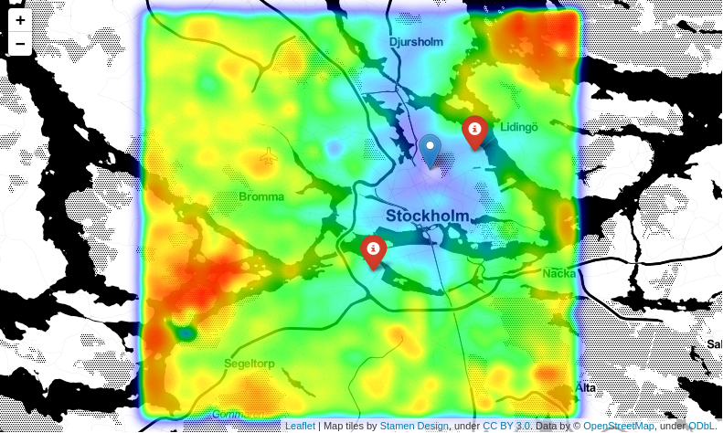
We can plot the travel-time map for the hobby (marked with a red marker) as follows:
plot_time_map(additional_markers=[{'string': 'Hobby',
                                   'latitude': hobby_lat,
                                   'longitude': hobby_long}],
              data=hobby_df)
In order to combine this data with the previous travel-time data, we join the two datasets:
merged_df = pd.merge(travel_df,
                     hobby_df,
                     on=['latitude', 'longitude'],
                     suffixes=['_work', '_hobby'])

merged_df.head()
| latitude | longitude | time_work | time_hobby | |
|---|---|---|---|---|
| 0 | 59.408582 | 17.854205 | 63.0 | 62.0 |
| 1 | 59.408582 | 17.862417 | 76.0 | 53.0 |
| 2 | 59.408582 | 17.870628 | 56.0 | 90.0 |
| 3 | 59.408582 | 17.878840 | 55.0 | 89.0 |
| 4 | 59.408582 | 17.887051 | 69.0 | 59.0 |
Now we can plot the locations on the map from which we can travel to either work
or the hobby within time minutes (these have both time_work <= time and
time_hobby <= time):
def plot_intersected_isochrone(time):
    intersected_isochrone = merged_df[(merged_df['time_work'] <= time) &
                                      (merged_df['time_hobby'] <= time)]

    map = folium.Map(
        location = [(sthlm_lat_start + sthlm_lat_stop) / 2,
                    (sthlm_long_start + sthlm_long_stop) / 2],
        tiles='Stamen Toner',
        zoom_start=11
    )

    marker_str = 'Work'
    folium.Marker([work_lat, work_long],
                  popup=marker_str,
                  tooltip=marker_str).add_to(map)

    marker_str = 'Hobby'
    folium.Marker([hobby_lat, hobby_long],
                  popup=marker_str,
                  icon=folium.Icon(color='red'),
                  tooltip=marker_str).add_to(map)


    HeatMap(intersected_isochrone[['latitude', 'longitude']].to_numpy(),
            min_opacity=0.5,
            max_val=time,
            radius=12,
            blur=11,
            max_zoom=10,
            gradient={1.0:'#00AA00', 0.0:'#00FF00'}
            ).add_to(map)

    return map
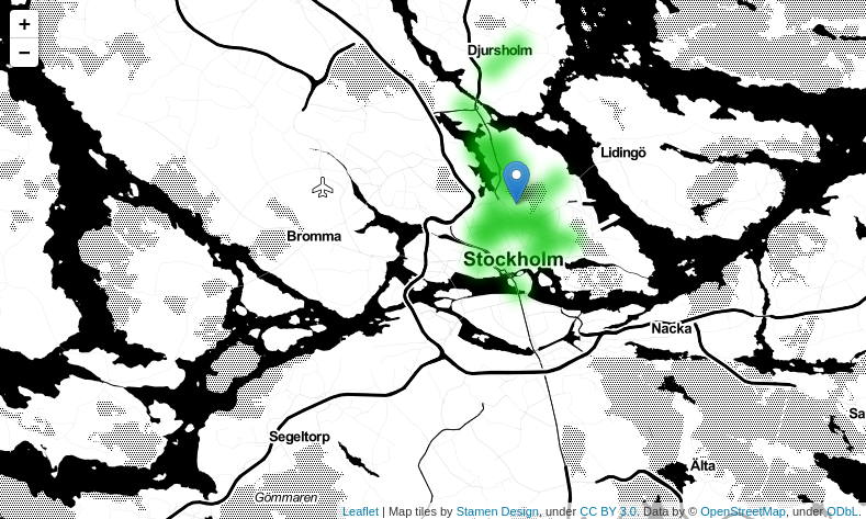
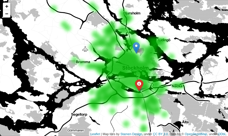
Feasible locations for relocation
The locations from which both the workplace (blue) and the hobby (red) can be reached within half an hour are:
plot_intersected_isochrone(30)
That essentially limits us to the very center of Stockholm – expensive!
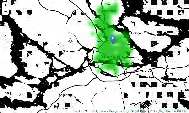
If we are a bit more flexible and allow for 45 minutes to either location, we obtain many more feasible locations:
plot_intersected_isochrone(45)
For reference, here is a geographic map of Stockholm with the railbound lines of public transport shown:
![]()
Note that it is not enough to live on a line; we need to live close to a station so as to have a short walking distance before we enter the public transport system – hence the isolated green spots close to Farsta, Kista, Tensta, etc. in the plot above.
Conclusion
In this post, we considered the problem of finding suitable locations to relocate to. In particular, we aimed to find locations from which we can travel to work – and perhaps also to a hobby – within a certain amount of time using the public transport system of Stockholm.
To do so, we first used the open API provided by Trafiklab to access travel-time data. We then visualized the data using Folium. From the visualizations, we noted that distance is not always a good proxy for travel time: just because two locations are close on a map, does not mean that they are close “in time”.
Finally, by combining travel-time data for both the workplace and the hobby, we obtained an answer to the question we set out to answer: what are feasible locations to consider for relocation (with respect to travel times)? This gives us a basis (and limits our search) for further investigations that take other important factors into account (price, neighborhood, etc.).
Extensions
This post was a weekend experiment and should be read as a fun proof-of-concept –
do not go and buy an apartment just because plot_intersected_isochrone(30) puts a green
spot there!
There is obviously a lot that could be improved and many extensions that are possible. Here are some ideas:
-
In order to maximize the amount of information one can obtain, while respecting the quota on the number of queries, one could come up with smarter ways of sampling the map (instead of the naive uniform grid).
-
For example, exclude coordinates that lie in the water, since there is obviously no house to which you could relocate there. The API seems to return data even for such locations – perhaps it computes the time from closest point on land?
-
Increase the
numBandnumFfields in the API-query to request more than one trip suggestion for the query. Then compute the min/mean/median of the returned travel times. This would help create a smoother travel-time plot. One could also compute an average over several days and/or times during a day for a more representative value. -
Use the Booli API to check if there are any apartments for sale in any of the feasible locations. One could also filter for underpriced objects (with respect to our conditions on travel times).
I hope that you enjoyed reading this post – if you have any comments, feel free to email me!